Creating a spycon test

In this notebook we demonstrate, how a test can be created, and immediately used for benchmarking. For simplicity, we reconstruct the same test, that is already in the data folder. Let’s load all the information, we need for a connectivity test. That means the

1. Spike train data (spike times & unit ids)

2. Set of units, that have been recorded

3. An array with three columns (pre unit id, post unit id, conn value). A row is one connection.

As conn value 0 means no synapse, otherwise it is a synapse. If it is nan for a connection pair is not indicated at all, it is assumed to be unknown and not considered for the metric computation.

import numpy
from matplotlib import pyplot

data = numpy.load('../data/gt_data/sim1917Cell1Block1_tiny.npz')
times, ids = data['times'], data['ids']
nodes = data['nodes']
marked_edges = data['marked_edges']

Now we have loaded all our the information we need, and we construct the ConnectivityTest object.

from spycon import ConnectivityTest
myconn_test = ConnectivityTest(name='MyTest', times=times, ids=ids, marked_edges=marked_edges, nodes=nodes)

Using cpu device

With the run_test method we can simply evaluated a connectivity algorithm on this test, and get sum interesting metrics.

from spycon import coninf
con_method = coninf.Smoothed_CCG()
metrics = myconn_test.run_test(con_method)

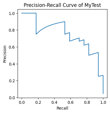
pyplot.figure(figsize=(4, 4))
pyplot.plot(metrics['prc_recall'][0], metrics['prc_precision'][0])
pyplot.xlabel('Recall')
pyplot.ylabel('Precision')
pyplot.title(f'Precision-Recall Curve of {myconn_test.name}')

100%|██████████| 380/380 [00:07<00:00, 51.93it/s]

Text(0.5, 1.0, 'Precision-Recall Curve of MyTest')

Test objects can be saved, and loaded easily.

from spycon import load_test

gt_data_path = '../data/gt_data/'
myconn_test.save(gt_data_path)

reloaded_test = load_test(name='MyTest', path=gt_data_path)